Quickstart with the single-resonator solver

Quickstart with the single-resonator solver#

Parameters initialization#

First, we need to import all the necessary libraries

import matplotlib.pyplot as plt
plt.rcParams['figure.dpi'] = 120
plt.rcParams['savefig.dpi'] = 120
import numpy as np
import sys,os
my_PyCore_dir = os.path.dirname('/Users/aleksandrtusnin/Documents/Projects/PyCORe/')
sys.path.append(my_PyCore_dir)
import PyCORe_main as pcm
from scipy.constants import c, hbar
%matplotlib widget

Then, we define the dispersion parameters:

Number of frequency modes used in the simulations
Array of comb indexes $\mu$

Num_of_modes = 2**9
mu = np.arange(-Num_of_modes/2,Num_of_modes/2)

Group velocity dispersion $D_2 = -\beta_2 \frac{D_1^2 c}{n_g}$ [$2\pi$Hz], where $D_1 = 2\pi FSR$

D2 = 4.1e6*2*np.pi

that then defines the integrated dispersion profile $D_\mathrm{int} = D_2 \frac{\mu^2}{2}$

Dint = (mu**2*D2/2) 

Note: higher order dispersion terms

To take into account higher order dispersion orders, you just need to define $D_3,\, D_4,...$ and redefine $D_\mathrm{int} = D_2 \frac{\mu^2}{2} + D_3 \frac{\mu^3}{3!} + D_4 \frac{\mu^4}{4!} + ...$

Note: mode crossings

Mode crossings can be added manually in the dispersion array as follows

mu_AMX = 35
Dint[mu_AMX]-=2*np.pi*1e6

In this example, we shifted the mode $\mu=35$ by $1$ GHz below the ‘unperturbed’ dispersion curve

Then, we create a dictionary with the physical parameters

PhysicalParameters = {'n0' : 1.9,
                      'n2' : 2.4e-19,### m^2/W
                      'FSR' : 181.7e9 ,
                      'w0' : 2*np.pi*192e12,
                      'width' : 1.5e-6,
                      'height' : 0.85e-6,
                      'kappa_0' : 50e6*2*np.pi,
                      'kappa_ex' : 50e6*2*np.pi,
                      'Dint' : Dint,
                      'Raman time' :  1e-15 #s
                      }

Further, we define the pump laser parameters, such as pump power, tuning range, and the scan time. We define the pump in the frequency domain within fftshift framework.

dNu_ini = -1e9 #Hz
dNu_end = 3e9 #Hz
nn = 2000
dOm = 2*np.pi*np.linspace(dNu_ini,dNu_end,nn)
scan_time = 1e-6 #s
P0 = 0.15### W
Pump = np.zeros(len(mu),dtype='complex')
Pump[0] = np.sqrt(P0)

Finally, we define the simulation parameters

simulation_parameters = {'slow_time' : scan_time,
                         'detuning_array' : dOm,
                         'noise_level' : 1e-9,
                         'output' : 'map',
                         'absolute_tolerance' : 1e-10,
                         'relative_tolerance' : 1e-6,
                         'max_internal_steps' : 2000}

simulation_parameters note

‘noise_level’ defines the amplitude of the white noise in the frequency domain;
‘output’ : ‘map’ defines the dense output from the solver: the result will be np.array([dOm.size,mu.size],dtype=complex). Alternative paramet is ‘fin_res’, that results only in the output of the final state at dOm[-1].
‘absolute_tolerance’, ‘relative_tolerance’, and ‘max_internal_steps’ define the condition for the step-adaptative solver

Class initialization#

Now, we need to initialize the resonator class from the Physical parameters

single_ring = pcm.Resonator()
single_ring.Init_From_Dict(PhysicalParameters)

Simulations#

We are ready to run our simulations

try:
    map2d = single_ring.Propagate_PseudoSpectralSAMCLIB(simulation_parameters, Pump,dt=0.5e-3)# only works if C libraries are installed
except: 
    map2d = single_ring.Propagate_SplitStep(simulation_parameters, Pump,dt=0.5e-3)# works with just Python

Normalized pump power $f_0^2$ = 33.0
Normalized detuning $\zeta_0$ = [-20.000000000000004,60.0]
f0^2 = 33.0
xi [-20.000000000000004,60.0]
J = 0.0
Progress: |██████████████████████████████████████████████████| 100.0% Complete, elapsed time = 36.3 s

Simulations print output

For convinience, normalized pump power $f_0^2$ and the detuning array $\zeta_0$ are printed before the execution.
Third line specifies the type of the solver that is used
4th and 5th lines reflect the building of the solver class
6th line represnts the progress bar

Data analysis#

Now the simulation results are storred in the array map2d that has the size [dOm.size $\times$ mu.size ] and contains the amplitude and the phase of the optical field envelope. Number of photons, storred in the cavity, defined as

np.sum(map2d,axis=1)/Num_of_modes

while number of modes for a comb line $\mu$ is

map2d[:,mu]/Num_of_modes

Transmission trace#

Dynamcis of the number of modes as detuning function presented below

Num_of_photons = np.sum(np.abs((map2d[:,:])/(Num_of_modes))**2,axis=1)
fig = plt.figure(frameon=False,dpi=150)
ax = fig.add_subplot(1,1,1)
ax.plot(dOm/2/np.pi/1e9,Num_of_photons)
ax.set_xlabel('Laser detuning (GHz)')
ax.set_ylabel('Number of photons')
ax.grid(True)
plt.show()

Transmission trace through the resonator can be obtained via

\[S_\mathrm{out} = S_\mathrm{in} - \sqrt{\kappa_\mathrm{ex}}A,\]

where $S_\mathrm{in}^2 = P_\mathrm{in}/\hbar\omega$ to $\mu$-th comb line and $A =$ map2d[:,mu]/Num_of_modes.

Below we show the simulated transmission trace that should be visible on a photodetector

Sin = Pump/np.sqrt(hbar*PhysicalParameters['w0'])
Sout = np.zeros_like(map2d)
Sout = Sin - np.sqrt(single_ring.kappa_ex)*map2d/Num_of_modes
fig = plt.figure(frameon=False,dpi=150)
ax = fig.add_subplot(1,1,1)
ax.plot(dOm/2/np.pi/1e9,np.sum(abs(Sout)**2,axis=1)/abs(Sin[0])**2)
ax.set_xlabel('Laser detuning (GHz)')
ax.set_ylabel('Normalized transmission')
plt.show()

Optical spectrum#

A simulated OSA spectrum for a given detuning can be presented as

Note

$|S_\mathrm{out}|^2\hbar\omega$ is measured in Watts, so to present it in dBm is pretty straightforward $$ \mathrm{Spectrum [dBm ]} = 10log_{10}(|S_\mathrm{out}|^2\hbar\omega/10^{-3}) $$

fig = plt.figure(frameon=False,dpi=150)
ax = fig.add_subplot(1,1,1)
ax.vlines(mu,-300,10*np.log10(np.abs(np.fft.fftshift(Sout[1000,:]))**2*hbar*PhysicalParameters['w0']/1e-3),lw=1.0)
ax.scatter(mu,10*np.log10(np.abs(np.fft.fftshift(Sout[1000,:]))**2*hbar*PhysicalParameters['w0']/1e-3),s=2.0)
ax.set_xlabel('Mode index $\mu$')
ax.set_ylabel('OSA spectrum (dBm)')
ax.set_ylim(-75,25)
ax.set_xlim(-120,120)
plt.show()

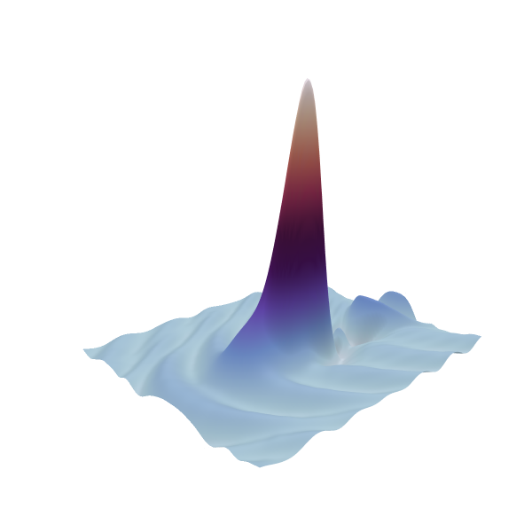
Quick dynamics plot#

To quickly analyze the generated data, we implemeted an interactive function Plot_map that allows for investigation of the field with different detuings

pcm.Plot_Map(np.fft.ifft(map2d,axis=1),dOm/2/np.pi/1e9,xlabel='Detuning', units='GHz')