Two coupled resonators

Two coupled resonators#

Parameters initialization#

We import all the necessary libraries in the usual way

import matplotlib.pyplot as plt
plt.rcParams['figure.dpi'] = 150
plt.rcParams['savefig.dpi'] = 150
import numpy as np
import sys,os
my_PyCore_dir = os.path.dirname('/Users/aleksandrtusnin/Documents/Projects/PyCORe/')
sys.path.append(my_PyCore_dir)
import PyCORe_main as pcm
from scipy.constants import c, hbar
%matplotlib widget

For simplicity, we define the same dispersion for both resonators.

Num_of_modes = 2**9
mu = np.arange(-Num_of_modes/2,Num_of_modes/2)
N_res = 2
Dint = np.zeros([Num_of_modes,N_res])
D2 = 4.1e6*2*np.pi
Dint[:,0] = (mu**2*D2/2) 
Dint[:,1] = (mu**2*D2/2) 

Different resonators dispersion

It can be readily implemeted via

Dint[:,0] = (mu**2*D2_1/2) 
Dint[:,1] = (mu**2*D2_2/2) 

Defferent FSR

Let’s define the difference as \(\Delta D_1\), then it can be readily taken intro account in the dispersion as

Dint[:,0] = (mu**2*D2_1/2) 
Dint[:,1] = (mu*DeltaD1 + mu**2*D2_2/2) 

Resonators often have different absolute frequencies, and we usually call it as intra-resonator detuning \(\Delta\). This value depends on the material and fabrication. However, with photonic Damascene and subtractive processes it can exceed tens of GHz. Here, we detune second resonator by \(0.01\) GHz with respect to the first.

Delta = np.zeros([Num_of_modes,(N_res)])

Delta[:,1] = 2*np.pi*0.01e9*np.ones([Num_of_modes])

The evanescent coupling \(J\) depends on the the resonators’ geometry and on the distance between them. Usually, this value can be extractred from, for example, Lumerical simulations, or experiment. In PyCORe, we define it as

J = 2*1e9*2*np.pi*np.ones([mu.size,(N_res-1)])

Frequency dependent coupling

In this particular example we defined the coupling to be frequency independent, however it’s not always the case. It often has exponential dependence on the mode number \(\mu\).

We define the couplings to the bus waveguides in the similar way

kappa_ex_ampl = 20e6*2*np.pi
kappa_ex = np.zeros([Num_of_modes,N_res])
kappa_ex[:,0] = kappa_ex_ampl*np.ones([Num_of_modes])
kappa_ex[:,1] = 2*kappa_ex_ampl*np.ones([Num_of_modes])

We finally define the resonator parameters to initialize the class

omega = 2*np.pi*193.414489e12

PhysicalParameters = {'Inter-resonator_coupling': J,
                      'Resonator detunings' : Delta,
                      'n0' : 1.9,
                      'n2' : 2.4e-19,### m^2/W
                      'FSR' : 457.9e9 ,
                      'w0' : omega,
                      'width' : 2.35e-6,
                      'height' : 0.8e-6,
                      'kappa_0' : 20e6*2*np.pi,
                      'kappa_ex' : kappa_ex,
                      'Dint' : Dint}
crow = pcm.CROW()
crow.Init_From_Dict(PhysicalParameters)

Pump laser parameters and detuning parameters are defined in the similar way as for just single resonator, except there is a possibility to pump different resonators

dNu_ini = -2*1e9
dNu_end = 3e9

nn = 1000
dOm = 2*np.pi*np.linspace(dNu_ini,dNu_end,nn)
simulation_parameters = {'slow_time' : 1e-6,
                         'detuning_array' : dOm,
                         'noise_level' : 1e-9,
                         'output' : 'map',
                         'absolute_tolerance' : 1e-10,
                         'relative_tolerance' : 1e-12,
                         'max_internal_steps' : 2000}

P0 = 0.3### W

Pump = np.zeros([len(mu),N_res],dtype='complex')

Pump[0,0] = np.sqrt(P0)

map2d = crow.Propagate_PSEUDO_SPECTRAL_SAMCLIB(simulation_parameters, Pump, BC='OPEN')

f0^2 = [5682.39    0.  ]
xi [-200.0,299.99999999999994] (normalized on $kappa_0/2)$
OPEN
Initializing pseudo spectral CROW
speudo spetral CROW is initialized
Step adaptative pseudo-spectral Dopri853  from NR3 without thermal effects is running
100% [||||||||||||||||||||||||||||||||||||||||||||||||||||||||||||]

Similar to the single resonator case from single-resonator example, we plot the transmission traces from both resonators

Sin = Pump/np.sqrt(hbar*PhysicalParameters['w0'])
Sout = np.zeros_like(map2d)
Sout = Sin - np.sqrt(crow.kappa_ex)*map2d/Num_of_modes

fig = plt.figure(figsize=[6,4],frameon=False,dpi=150)
ax = fig.add_subplot(1,2,1)
ax.plot(dOm[10:]/2/np.pi/1e9,np.sum(abs(Sout[10:,:,0])**2,axis=1)/np.max(abs(Sin)**2),label='1$^{\mathrm{th}}$ resonator')
ax.set_ylabel(r'Transmission $S_\mathrm{out}/S_\mathrm{in}$')
ax.set_xlabel('Pump detuning (GHz)')
plt.legend()
ax = fig.add_subplot(1,2,2)
ax.plot(dOm[10:]/2/np.pi/1e9,np.sum(abs(Sout[10:,:,1])**2,axis=1)/np.max(abs(Sin)**2),c='r',label='2$^{\mathrm{nd}}$ resonator')
ax.set_xlabel('Pump detuning (GHz)')
plt.legend()
plt.tight_layout()

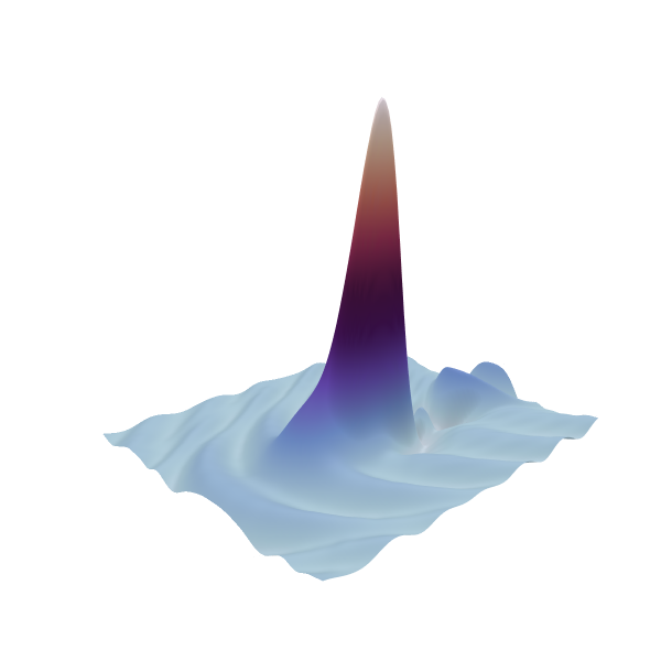
The function Plot_map can also be used to interactively investigate resonator dynamics.

pcm.Plot_Map(np.fft.ifft(Sout[:,:,1],axis=1),np.arange(dOm.size),xlabel='Detuning index', units='')

Two coupled resonators

Contents

Two coupled resonators#

Parameters initialization#